Examples contain material we will discuss and use to learn R in class. These notes are not comprehensive. Instead, they are meant as a helpful resource during and after class in case you are confused or have trouble remembering something we discussed.
Getting started with R and RStudio
R is not a programming language like C or Java. It was not created by software engineers for software development. Instead, it was developed by statisticians as an interactive environment for data analysis. This interactivity makes it easy to explore data quickly, which is an indispensable feature for many tasks in business analytics, statistics, data science, and other fields.
If you have prior programming experience, you may be surprised by differences between R and other programming languages.
If you have no prior programming experience, you may initially be frustrated when learning R. That is normal! Learning to program is essentially learning to speak a new language. But in some ways it’s even more difficult, because your interlocutor is a computer who isn’t always great at telling you when you said something that made no sense.
Regardless of your prior experience, if you are patient, you will come to appreciate the power of R for data analysis and data visualization.
R, and the R console
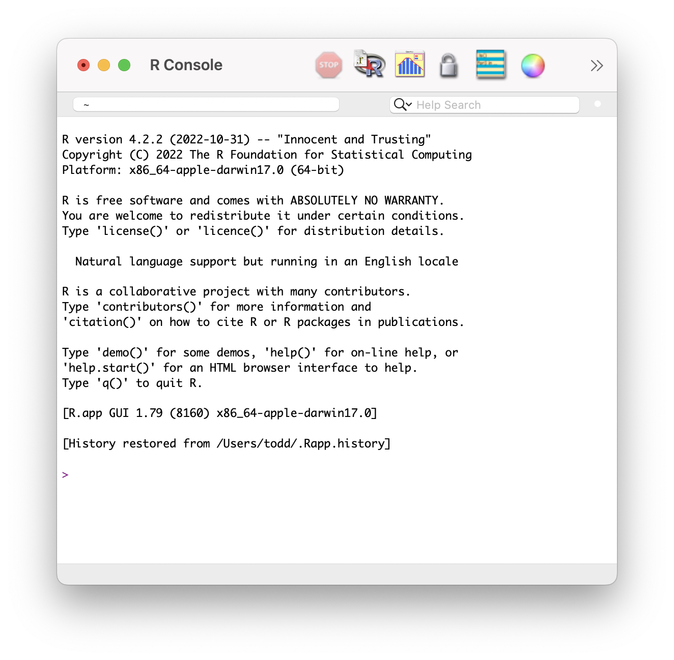
You can think of R analogously to the engine in a car: it will power our work. One way to control that engine is to use the R console to execute commands as you type them, or to run scripts you have already written. There are several ways to gain access to the R console. One way is to install R on your computer and open the built-in console, which looks like this:

However, most people don’t use this console. Instead, they use an integrated development environment (or IDE) to write, debug, and execute their code.
RStudio
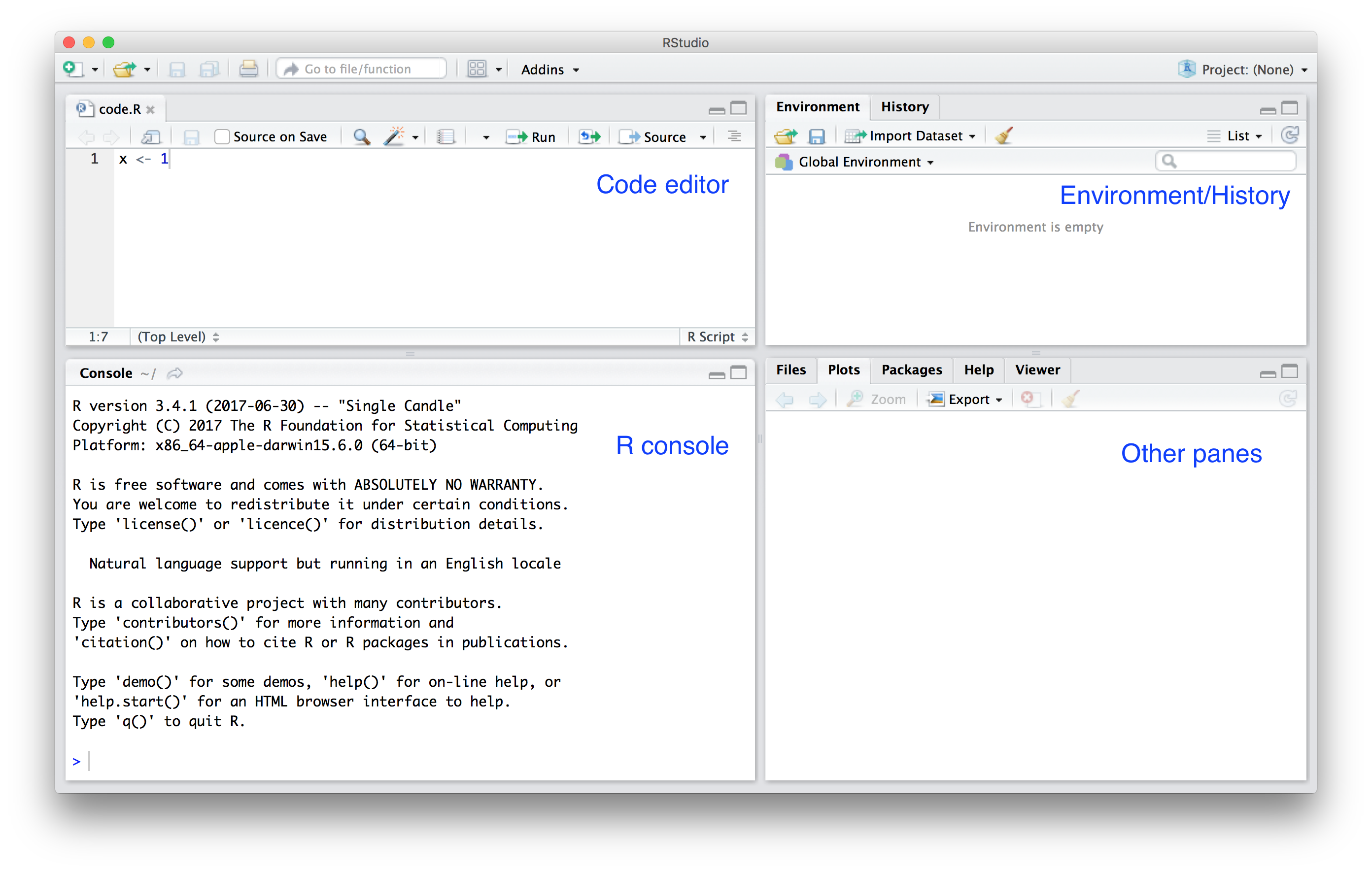
The IDE we will use in this class is RStudio. RStudio includes an editor with many R-specific features, a console to execute your code, and other useful panes, including one to show figures or view html documents you produce. RStudio looks like this:

RStudio will be our launching pad for data science projects. You can think of it as the dashboard in your car. It not only provides an editor for us to create and edit our scripts but also provides many other useful tools. In this section, we go over some of the basics.
RStudio panes
When you start RStudio for the first time, you will see three panes by default. The left pane shows the R console. On the right, the top pane includes tabs such as Environment and History, while the bottom pane shows six tabs: File, Plots, Packages, Help, Viewer, and Presentation (these tabs may change in new versions). You can click on each tab to move across the different features.
To start a new R script, you can click on File, then New File, then R Script.
This starts a new pane on the left and it is here where you can start writing your script.
Keyboard shortcuts
Many tasks we perform with the mouse can be achieved with a combination of key strokes instead, or keyboard shortcuts For example, we just showed how to use the mouse to start a new script, but you can also use a shortcut: Ctrl+⇧+N on Windows and ⌘+⇧+N on macs.
Although using the mouse to explore RStudio’s dropdown menus is a good place to start, I highly recommend that you memorize key bindings for the operations you use most. RStudio provides a useful cheat sheet with the most widely used commands. If you’re on a mac, you can access a list of keyboard by pressing ⌥+⇧+K. You might want to keep this in mind so you can look up keyboard shortcuts when you find yourself doing the same point-and-click operations repeatedly.
Tab completion
One advantage of using RStudio is that it has context-aware tab completion. This means that when you start typing the name of a package, function, or object you want to use, RStudio will automatically suggest ways to complete your input. You can take advantage of this by scrolling through the suggestions using up/down arrows and hitting tab to use the selected completion.
RStudio also does handy things like adding a close parentheses when you type an open parentheses, such as if you type library(.
Running commands while editing scripts
There are many editors specifically made for coding. These are useful because color and indentation are automatically added to make code more readable. RStudio is one of these editors, and it was specifically developed for R. One of the main advantages provided by RStudio over other editors is that we can test our code easily as we edit our scripts.
You can see this by opening a new script. Give the script a name. You can do this through the editor by saving the current new unnamed script. To do this, click on the save icon or use the key binding Ctrl+S on Windows and ⌘+S on the Mac.
When you ask for the document to be saved for the first time, RStudio will prompt you for a name. A good convention is to use a descriptive name, with lower case letters, no spaces, only hyphens to separate words, and then followed by the suffix .R. Call your script my-first-script.R.
Now we are ready to start editing our first script. For example, you could write:
print("welcome to RStudio")
If you do this and hit ↩︎ in the editor, nothing will happen in the console.
To execute your new script, you can click on the Run button on the upper right side of the editing pane or use the keyboard shortcut: Ctrl+⇧+↩︎ on Windows or ⌘+⇧+↩︎ on Mac. When you do this, the console will show the command as well as its output:
## [1] "welcome to RStudio"
To run one line at a time instead of the entire script, you can use Ctrl+↩︎ on Windows and ⌘+↩︎ on Mac.
Quarto / R Markdown
Note: Quarto is an authoring framework that extends R Markdown. If you are familiar with R Markdown it will be easy to transition to Quarto.
Quarto provides a unified authoring framework for data science that combines your code, its results, and your prose commentary. Quarto documents are fully reproducible and support dozens of output formats, like PDFs, Word files, slideshows, and more.
Quarto files are designed to be used in three ways:
For communicating to decision makers, who want to focus on the conclusions, not the code behind the analysis.
For collaborating with others (including future you!) who are interested in your conclusions and how you reached them.
As an environment in which to do business analytics, where you can capture not only what you did, but also what you were thinking.
All three of these are relevant for this course. Hopefully you can see how the first could be useful in business settings where you need to present a summary of ideas or findings to a decision maker.
quarto.org provides many more resources to help you as you begin to work with Quarto.
You may also find the Quarto cheatsheet helpful when getting started.
Quarto basics
Quarto files contain three types of content:
- An (optional) YAML header surrounded by
---s.
- Chunks of R code surrounded by
```.
- Text mixed with simple text formatting like
# heading and _italics_.
You can edit each of these to affect the final output.
When you are done composing your document, you can render it by clicking Render or by using the keyboard shortcut ⌘+⇧+K. This will process the file through several steps to produce your output in the format you specify.
Markdown basics
Markdown is a set of formatting conventions for plain text files that is widely used (beyond R). We will use an example file on RStudio Cloud to learn about some basic text formatting using Markdown. You can also read more about this in R for Data Science (2e).

