Data import and tidying

class: center middle main-title section-title-4

# Data import and tidying

.class-info[

**Week 3**

AEM 2850 / 5850 : R for Business Analytics<br>
Cornell Dyson<br>
Fall 2025

Acknowledgements: 


[Grant McDermott](https://github.com/uo-ec607/lectures),
[Allison Horst](https://github.com/allisonhorst/stats-illustrations),
[R4DS (2e)](https://r4ds.hadley.nz/data-tidy.html)

]

---

# Announcements

Submit assignments via gradescope
- Either via canvas or directly in gradescope
- Homework - Week 2 was due yesterday (Monday) at 11:59pm

We will not assign any late penalties for the survey and homework-02

Late assignments will be penalized going forward
- If something comes up, please email me, Victor, and Xiaorui **in advance**

Questions before we get started?

---

# Plan for this week

.pull-left[
### Tuesday
[Prologue](#prologue)

[Data import](#readr)
  - [read_csv](#read_csv)
  - [write_csv](#write_csv)
  - [read_excel](#read_excel)

[example-03-1](#example-1)
]

.pull-right[
### Thursday
[Tidy data](#tidyr)
  - [pivot_longer](#pivot_longer)
  - [pivot_wider](#pivot_wider)

[Summary](#summary)

[example-03-2](#example-2)
]

---
class: inverse, center, middle
name: prologue

# Prologue

---

# What are our concentrations?

Take a guess: what's the most common concentration among classmates?

Let's figure this out using the course survey

First, let's **import** the data:

``` r
responses <- read_csv("data/survey-responses/homework-1-survey.csv")
```

```
## Rows: 114 Columns: 22
## ── Column specification ────────────────────────────────────────────────────────
## Delimiter: ","
## chr (22): Timestamp, Email Address, Name, netid, Name pronunciation guide (o...
## 
## ℹ Use `spec()` to retrieve the full column specification for this data.
## ℹ Specify the column types or set `show_col_types = FALSE` to quiet this message.
```

---

# What are our concentrations?

``` r
responses |> 
  select(Concentration)
```

```
## # A tibble: 114 × 1
##    Concentration                    
##    <chr>                            
##  1 Finance                          
##  2 Finance                          
##  3 Business Analytics and Accounting
##  4 Business Analytics               
##  5 Entrepreneurship                 
##  6 Entrepreneurship                 
##  7 Finance                          
##  8 Strategy                         
##  9 Business Analytics               
## 10 Business Analytics               
## # ℹ 104 more rows
```

What is the "level of observation" in this data frame? (i.e., what are the rows?)

---

# What are our concentrations?

After some processing to get concentration counts, we get:

```
## # A tibble: 1 × 12
##    acct    ba   dev  econ  entr enviro finance  food  mgmt  mktg other strategy
##   <int> <int> <int> <int> <int>  <int>   <int> <int> <int> <int> <int>    <int>
## 1     6    20     5     7     6      3      39    10     3     9     3       10
```

What is the "level of observation" in this data frame? (i.e., what are the rows?)

Is the best way to organize concentration counts?

How would you use counts to compute shares in this data frame?

---

# What are our "tidy" concentrations?

.pull-left[
Let's `pivot_longer` and `slice_max` to get the top 3:
]

.pull-right[
How would you use what we learned last week to compute shares?
]

.pull-left[

```
## # A tibble: 4 × 2
##   concentration count
##   <chr>         <int>
## 1 finance          39
## 2 ba               20
## 3 food             10
## 4 strategy         10
```
]

.pull-right[

``` r
tidy_concentrations |> 
  mutate(share = count / sum(count))
```

```
## # A tibble: 4 × 3
##   concentration count  share
##   <chr>         <int>  <dbl>
## 1 finance          39 0.322 
## 2 ba               20 0.165 
## 3 food             10 0.0826
## 4 strategy         10 0.0826
```
]

---
class: inverse, center, middle
name: readr

# Data import

---

# Data import

Plain-text rectangular files are a common way to store and share data:
- comma delimited files (`readr::read_csv`)
- tab delimited files (`readr::read_tsv`)
- fixed width files (`readr::read_fwf`)

We will just cover csv files since `readr` syntax is transferable

---

# Super bowl ads: a csv example

???
Image source: [FiveThirtyEight](https://github.com/fivethirtyeight/superbowl-ads)

---

# Super bowl ads in csv format

???
Data source: [FiveThirtyEight](https://github.com/fivethirtyeight/superbowl-ads)

---

# Super bowl ads in csv format

---

# Getting from a csv to a data frame

How are data frames and csv files similar?

--
- both are rectangular
- csv lines often correspond to rows
- csv commas delineate columns

How are they different?

--
- csv files do not store column types!

---
name: read_csv

# 1) readr::read_csv

`read_csv` helps us get from point a to point b:
1. you give it the path to your csv file
2. it takes the first line of data as column names by default
3. it guesses column types and builds up a data frame

Most csv files can be read using the defaults, so we will focus on that

If you run into special cases, consult `?read_csv`

---

# An aside on paths

We need to figure out what "path" to give `read_csv` to get to our file

The simplest thing is to provide a "relative path" from the working directory

**But where is the working directory?**

**R scripts (.R)** in an R Project: default working directory is the project directory

**Quarto (.qmd)**: default working directory is the location of the .qmd file

In our RStudio Cloud projects, these will both be `/cloud/project`, which is the default directory for our projects and where we store our .qmd templates

---

# 1) readr::read_csv

Here is an example for the file `superbowl.csv` inside the folder `data`:

``` r
ads <- read_csv("data/superbowl.csv")
```

```
## Rows: 247 Columns: 25
## ── Column specification ────────────────────────────────────────────────────────
## Delimiter: ","
## chr  (10): brand, superbowl_ads_dot_com_url, youtube_url, id, kind, etag, ti...
## dbl   (7): year, view_count, like_count, dislike_count, favorite_count, comm...
## lgl   (7): funny, show_product_quickly, patriotic, celebrity, danger, animal...
## dttm  (1): published_at
## 
## ℹ Use `spec()` to retrieve the full column specification for this data.
## ℹ Specify the column types or set `show_col_types = FALSE` to quiet this message.
```

That was easy!

???
Note: readr intentionally never guesses that columns are integers as a safeguard ([source](https://github.com/tidyverse/readr/issues/1094#issuecomment-628612430))

---

# Now we're back to our old tricks

.less-left[

``` r
ads |> 
  count(funny)
```

```
## # A tibble: 2 × 2
##   funny     n
##   <lgl> <int>
## 1 FALSE    76
## 2 TRUE    171
```
]

.more-right[

``` r
ads |> 
  group_by(brand) |> 
  summarize(likes = sum(like_count, na.rm = TRUE)) |> 
  arrange(desc(likes))
```

```
## # A tibble: 10 × 2
##    brand      likes
##    <chr>      <dbl>
##  1 Doritos   326151
##  2 NFL       224263
##  3 Coca-Cola 160231
##  4 Bud Light 104380
##  5 Budweiser  88765
##  6 Pepsi      14796
##  7 Toyota      5316
##  8 Hynudai     4204
##  9 E-Trade     2624
## 10 Kia         2127
```
]

---
name: write_csv

# 2) readr::write_csv

Use `write_csv` to write data to a `.csv`:

``` r
# overwrite the raw data (bad idea!)
ads |> 
  write_csv("data/superbowl.csv")
```

``` r
# modify the data and then output it to a new file
ads |> 
  select(year, brand, youtube_url) |> 
  write_csv("superbowl-urls.csv")
```

---
name: read_excel

# Importing excel data

Wait, what about getting data from excel spreadsheets?

Use `readxl::read_excel()` for data that is stored in `.xls` or `.xlsx` format

`readxl` isn't loaded as part of the core tidyverse, so we need to load it first:

``` r
library(readxl) # already installed as part of the tidyverse, but not loaded by default
read_excel("data/readxl/datasets.xlsx", sheet = "mtcars") |> head()
```

```
## # A tibble: 6 × 11
##     mpg   cyl  disp    hp  drat    wt  qsec    vs    am  gear  carb
##   <dbl> <dbl> <dbl> <dbl> <dbl> <dbl> <dbl> <dbl> <dbl> <dbl> <dbl>
## 1  21       6   160   110  3.9   2.62  16.5     0     1     4     4
## 2  21       6   160   110  3.9   2.88  17.0     0     1     4     4
## 3  22.8     4   108    93  3.85  2.32  18.6     1     1     4     1
## 4  21.4     6   258   110  3.08  3.22  19.4     1     0     3     1
## 5  18.7     8   360   175  3.15  3.44  17.0     0     0     3     2
## 6  18.1     6   225   105  2.76  3.46  20.2     1     0     3     1
```

---
class: inverse, center, middle
name: example-1

# example-03-1:<br>import-data-practice.R

---
class: inverse, center, middle
name: tidyr

# Tidy data

---

---

# *Why* "tidy" data?

---

---

# Which of these do you think is most tidy?

.pull-left.small[

``` r
table1
#> # A tibble: 4 × 4
#>   country      year  cases population
#>   <chr>       <dbl>  <dbl>      <dbl>
#> 1 Afghanistan  1999    745   19987071
#> 2 Afghanistan  2000   2666   20595360
#> 3 Brazil       1999  37737  172006362
#> 4 Brazil       2000  80488  174504898
```

``` r
table3
#> # A tibble: 4 × 3
#>   country      year rate             
#>   <chr>       <dbl> <chr>            
#> 1 Afghanistan  1999 745/19987071     
#> 2 Afghanistan  2000 2666/20595360    
#> 3 Brazil       1999 37737/172006362  
#> 4 Brazil       2000 80488/174504898  
```
]

.pull-right.small[

``` r
table2
#> # A tibble: 8 × 4
#>   country      year type           count
#>   <chr>       <dbl> <chr>          <dbl>
#> 1 Afghanistan  1999 cases            745
#> 2 Afghanistan  1999 population  19987071
#> 3 Afghanistan  2000 cases           2666
#> 4 Afghanistan  2000 population  20595360
#> 5 Brazil       1999 cases          37737
#> 6 Brazil       1999 population 172006362
#> # … with 2 more rows
```
]

Here, `table1`. Though in general, it can depend on your objectives!

---

# Why is `table1` a good choice?

The `dplyr` functions from last week are designed to work with tidy data:

.pull-left[

``` r
# compute rate per 10,000 people
table1 |>
  mutate(rate = cases / population * 10000)
```

```
## # A tibble: 4 × 5
##   country      year cases population  rate
##   <chr>       <dbl> <dbl>      <dbl> <dbl>
## 1 Afghanistan  1999   745   19987071 0.373
## 2 Afghanistan  2000  2666   20595360 1.29 
## 3 Brazil       1999 37737  172006362 2.19 
## 4 Brazil       2000 80488  174504898 4.61
```
]

.pull-right[

``` r
# compute cases per year
table1 |>
  group_by(year) |> 
  summarize(cases = sum(cases))
```

```
## # A tibble: 2 × 2
##    year cases
##   <dbl> <dbl>
## 1  1999 38482
## 2  2000 83154
```
]

---

# Why is `table1` a good choice?

The `ggplot2` functions we will learn are designed to work with tidy data:

.pull-left[

``` r
# visualize changes over time
table1 |> 
  ggplot(aes(
    x = year, 
    y = cases,
    color = country
    )) +
  geom_line() +
  geom_point() +
  scale_x_continuous(breaks = c(1999, 2000)) +
  theme_bw() +
  theme(legend.position = "bottom")
```
]

.pull-right[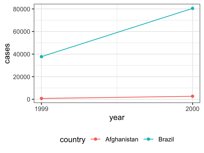
  ![](03-slides_files/figure-html/ggplot2-example-1.png)
]

---

# *How* can we "tidy" data?

**Key tidyr verbs**

1. `pivot_longer`: Pivot wide data into long format

2. `pivot_wider`: Pivot long data into wide format

---
name: pivot_longer

# Let's start with an untidy dataset

``` r
stocks
```

```
## # A tibble: 2 × 4
##   date        AAPL  GOOG  MSFT
##   <date>     <dbl> <dbl> <dbl>
## 1 2025-09-15  234.  199.  412.
## 2 2025-09-14  236.  195.  364.
```

We have 4 columns, the date and the stocks

Why do I think this is untidy?

1. stock names `AAPL`, `GOOG`, `MSFT` are values, not variables
2. cells contain prices, but there is no variable `price`

---

# 1) tidyr::pivot_longer

Let's use `pivot_longer()` to get this in tidy form

We want to pivot the stock name columns `AAPL`, `GOOG`, `MSFT` "longer"

We need to give three key pieces of information to `pivot_longer()`:

1. **Which columns to pivot** using `c(AAPL, GOOG, MSFT)` or `-date`
2. **What variable will hold the names** using `names_to = "stock"`
3. **What variable will hold the values** using `values_to = "price"`

Here is what that syntax looks like:

``` r
stocks |> 
  pivot_longer(cols = c(AAPL, GOOG, MSFT), names_to = "stock", values_to = "price")
```

---

# 1) tidyr::pivot_longer

Here is what that syntax does:

``` r
stocks |> pivot_longer(cols = c(AAPL, GOOG, MSFT), names_to = "stock", values_to = "price")
```

```
## # A tibble: 6 × 3
##   date       stock price
##   <date>     <chr> <dbl>
## 1 2025-09-15 AAPL   234.
## 2 2025-09-15 GOOG   199.
## 3 2025-09-15 MSFT   412.
## 4 2025-09-14 AAPL   236.
## 5 2025-09-14 GOOG   195.
## 6 2025-09-14 MSFT   364.
```

Let's save the "tidy" (i.e., long) stocks data frame for later use

``` r
tidy_stocks <- stocks |> 
  pivot_longer(cols = -date, names_to = "stock", values_to = "price")
```

---

# 1) tidyr::pivot_longer: How does it work?

``` r
df |> 
  pivot_longer(
*   cols = c(col1, col2),
    names_to = "name",
    values_to = "value"
  )
```

.less-left[
Existing variables such as `var` need to be repeated, once for each column in `cols`
]

.more-right[
<img src="img/03/pivot-longer-variables.png" width="85%" style="display: block; margin: auto;" />
]

---

# 1) tidyr::pivot_longer: How does it work?

``` r
df |> 
  pivot_longer(
    cols = c(col1, col2),
*   names_to = "name",
    values_to = "value"
  )
```

.less-left[
Column names become values in a new variable, whose name is given by `names_to`
  - repeated once for each row in the original
]

.more-right[
<img src="img/03/pivot-longer-column-names.png" width="85%" style="display: block; margin: auto;" />
]

---

# 1) tidyr::pivot_longer: How does it work?

``` r
df |> 
  pivot_longer(
    cols = c(col1, col2),
    names_to = "name",
*   values_to = "value"
  )
```

.less-left[
Cell values become values in a new variable, with a name given by `values_to`
]

.more-right[
<img src="img/03/pivot-longer-cell-values.png" width="85%" style="display: block; margin: auto;" />
]

---
name: pivot_wider

# 2) tidyr::pivot_wider

We can use `pivot_wider()` to make data "wide"

Let's say we want to convert `tidy_stocks` back to `stocks`

.pull-left[

``` r
tidy_stocks
```

]

.pull-right[

``` r
stocks
```

```
## # A tibble: 2 × 4
##   date        AAPL  GOOG  MSFT
##   <date>     <dbl> <dbl> <dbl>
## 1 2025-09-15  234.  199.  412.
## 2 2025-09-14  236.  195.  364.
```

]

---

# 2) tidyr::pivot_wider

.less-left[

``` r
tidy_stocks
```

.more-right[
We need to give two key pieces of information to `pivot_wider()`:

1. **What variable to get names from:** `names_from = stock`
2. **What variable to get values from:** `values_from = price`

`pivot_wider()` figures out the rest
]

---

# 2) tidyr::pivot_wider

``` r
tidy_stocks |> pivot_wider(names_from = stock, values_from = price)
```

```
## # A tibble: 2 × 4
##   date        AAPL  GOOG  MSFT
##   <date>     <dbl> <dbl> <dbl>
## 1 2025-09-15  234.  199.  412.
## 2 2025-09-14  236.  195.  364.
```

We just got our original data back!

``` r
stocks
```

```
## # A tibble: 2 × 4
##   date        AAPL  GOOG  MSFT
##   <date>     <dbl> <dbl> <dbl>
## 1 2025-09-15  234.  199.  412.
## 2 2025-09-14  236.  195.  364.
```

---

# 2) tidyr::pivot_wider

Reversing the arguments effectively transposes the original data:

``` r
tidy_stocks |> pivot_wider(names_from = date, values_from = price)
```

```
## # A tibble: 3 × 3
##   stock `2025-09-15` `2025-09-14`
##   <chr>        <dbl>        <dbl>
## 1 AAPL          234.         236.
## 2 GOOG          199.         195.
## 3 MSFT          412.         364.
```

``` r
stocks
```

```
## # A tibble: 2 × 4
##   date        AAPL  GOOG  MSFT
##   <date>     <dbl> <dbl> <dbl>
## 1 2025-09-15  234.  199.  412.
## 2 2025-09-14  236.  195.  364.
```

---

# tidyr resources

[Data tidying with tidyr : : CHEATSHEET](https://rstudio.github.io/cheatsheets/tidyr.pdf)

[Vignette](https://cran.r-project.org/web/packages/tidyr/vignettes/tidy-data.html) (from the **tidyr** package)

``` r
vignette("tidy-data")
```

[Ch. 5 of R for Data Science (2e)](https://r4ds.hadley.nz/data-tidy)

[Original paper](https://vita.had.co.nz/papers/tidy-data.pdf) (Hadley Wickham, 2014 JSS)

---
class: inverse, center, middle
name: summary

# Summary

---

# Key verbs so far

.pull-left-3[
### Import
#### readr
1. `read_csv`
2. `write_csv`

#### readxl
1. `read_excel`
]

.pull-middle-3[
### Tidy
#### tidyr
1. `pivot_longer`
2. `pivot_wider`
]

.pull-right-3[
### Transform
#### dplyr
1. `filter`
2. `arrange`
3. `select`
4. `mutate`
5. `summarize`
]

---
class: inverse, center, middle
name: example-2

# example-03-2:<br>tidy-data-practice.R